The Hidden Mathematics of Football
Poisson, Voronoi, minimax, and ten thousand simulated Senegals: a complete theory of the most beautiful, and most random, game on Earth
Over seventy years, probability theory, statistics, geometry, game theory, and machine learning quietly became football's second language. Using the 2026 World Cup as a live laboratory, and FootDigest's own prediction engine as the narrative thread, this paper builds the complete mathematical theory of the game: from the Poisson structure of goals and the measured unpredictability of football, through Dixon–Coles ratings, Monte Carlo futures, the trigonometry of expected goals, Markov possession value, the geometry of space, and the minimax equilibrium of the penalty kick, to an honest account of where the mathematics ends.
The night I watched a distribution collapse: the live win probability for Senegal, minute by minute. It peaked near 92% at minute 79. It ended at zero. Drag across the chart to replay any moment.
“In football, the worst blindness is only seeing the ball.” Nelson Falcão Rodrigues
Prologue: Seattle, Minute 79
On the night of July 1st, 2026, in Seattle, I watched a probability distribution collapse in real time.
Senegal led Belgium 2–0 in the Round of 32 of the World Cup. My model, the one I’d been building for months into FootDigest, had gone into that match making them underdogs, barely a 31% chance against a stronger Belgium side. But a two-goal lead with ten minutes left rewrites the board. Not because the model loved Senegal (models don’t love anyone, which is both their virtue and their tragedy), but because history is brutally clear about what happens when a team leads by two goals that late in a knockout match: it holds on better than nine times in ten. It almost never loses.
Almost is the most important word in this entire paper.
Belgium scored twice in a three-minute span. Extra time. Then a penalty (chaotic, contested, the kind of decision that will be relitigated in Dakar living rooms for a decade) and it was over. Belgium 3, Senegal 2. The tail of the distribution had arrived, wearing red.
Here is the thing nobody tells you about building football prediction models: the moment they hurt you most is the moment they are working perfectly. A one-in-ten event is supposed to happen one time in ten. If it never happened, my model would be broken. And yet, sitting there watching Sadio Mané’s face at the final whistle, no part of me was consoled by calibration curves.
This paper is about that tension. It is about how, over seventy years, probability theory, statistics, geometry, game theory, and machine learning quietly became football’s second language, and about what that language can and cannot say. I will use this World Cup, the one still unfolding across North America as I write, as the laboratory. I will use FootDigest, the analytics platform I have been building through it, as the narrative thread, because there is no better way to understand these ideas than to have your own model publicly, painfully wrong. And I will try to hold this essay to the same standard I hold the product: real sourced numbers or honest absence. Every empirical claim below is either cited to a specific paper, drawn from this tournament’s public record, or explicitly labelled as illustrative.
We begin in the 1950s, with a statistician who noticed something strange about goals.
Three promises, so you know what you’re holding:
First, the mathematics is real. Where I give an equation, it is the actual equation, not a gesture at one. Where I simplify, I say so. The appendix contains a full specification of FootDigest’s model (its data, parameters, and validation protocol) in the format machine learning researchers call a model card, because a prediction you can’t audit is an opinion with extra steps.
Second, the claims are falsifiable. A probabilistic model earns trust in exactly one way: its 70% predictions must come true about 70% of the time, measured across hundreds of matches. I’ll show you the scoring rules that make that sentence precise, and where models, including mine, fall short.
Third, the football comes first. Every abstraction in this paper is anchored to a moment from this World Cup: a shot Nicolas Jackson put against the post in New York, a stoppage-time VAR decision that reordered Group G for the seventh time in an evening, two penalty shootouts on the same night that vindicated a theorem from 1928. If the mathematics ever stops illuminating the game and starts replacing it, I’ve failed, and you should say so in the comments.
Notation, once, so we never trip on it: λ (lambda) is an expected goal rate; α and β are a team’s attack and defence ratings; θ (theta) is a geometric angle; P(·) is a probability; E[·] is an expectation. That’s the whole alphabet we need.
PART I: RANDOMNESS
Why Football Is the Most Unpredictable Major Sport on Earth (Measurably)
I.1 · The horse kicks of the Prussian cavalry
In 1837, Siméon Denis Poisson published a treatise on the probability of judicial verdicts. Buried inside was a distribution describing rare, independent events occurring at a constant average rate. Ladislaus Bortkiewicz made it famous in 1898 by showing it perfectly described deaths by horse kick in the Prussian cavalry: events so rare, so independent, so steadily distributed that their chaos had a shape.
The Poisson distribution says: if events occur at an average rate λ per unit of exposure, the probability of observing exactly k events is
One parameter. The distribution’s mean is λ and (this is the signature) its variance is also λ. If you ever want to test whether some count process is Poisson, check whether its variance equals its mean. Hold that thought.
Where does this formula come from? It’s not arbitrary; it is what the binomial distribution becomes at the limit of rarity. Slice a football match into n tiny intervals, each with a small probability p = λ/n of containing a goal. The number of goals is binomial(n, p). Let n → ∞ while λ = np stays fixed (infinitely many moments, each almost never decisive) and the binomial converges to the Poisson. A football match is this limit made flesh: ninety-plus minutes of near-misses discretized into two or three actual events. The Poisson isn’t a model we impose on football. It is what football’s structure implies.
The first equation, made playable. Drag λ, the average goals per match, and watch the probability of each scoreline count redraw. Notice the mean and the variance stay equal, the distribution’s signature. At a World Cup’s λ ≈ 2.5, a 0–0 still lands about 8% of the time.
I.2 · 1956: the first person to check
The first person to actually test this against football data was M.J. Moroney [1] (1956). Facts from Figures. Penguin. The first serious statistical treatment of football scores; Poisson and negative binomial fits. , in his 1956 book Facts from Figures: fit a Poisson to English league scorelines and it works, well, though not perfectly. Real goal counts are slightly over-dispersed (variance a touch above the mean; the negative binomial fits the tail better), a wrinkle whose cause (teams differ in quality, and game states feed back into scoring rates) will drive the next fifty years of refinements. But as a first approximation, one number per team per match captures the scoring process of the world’s most complex team sport. This should be shocking. It gets more shocking.
Twelve years later came the field’s founding trauma. Charles Reep, a Royal Air Force accountant, had spent two decades hand-notating matches (hundreds of them, by pencil, in a private shorthand) and in 1968 published, with Bernard Benjamin, “Skill and Chance in Association Football” [2] (1968). Skill and Chance in Association Football. JRSS-A 131. The founding paper and the founding fallacy; read it alongside its critics as a permanent vaccine against denominator neglect. in the Journal of the Royal Statistical Society. Their headline finding: roughly 80% of goals came from moves of three passes or fewer. Reep’s conclusion: passing is overrated; get the ball forward fast. English football listened. The long-ball era, decades of it, traces intellectually to this paper.
The finding was true. The conclusion was false. Roughly 80% (more, in fact) of all possessions are three passes or fewer, so of course most goals come from them: short possessions dominate the denominator. Condition properly, and longer passing sequences convert at a higher rate per possession. Reep had discovered the base rate and mistaken it for an edge; football analytics was born holding the wrong end of a conditional probability.
I keep Reep’s story taped above my desk, metaphorically, while building FootDigest, because it is the field’s permanent cautionary tale: the data was right, the counting was right, and the inference destroyed a generation of English football. Descriptive statistics without probabilistic reasoning isn’t neutral. It’s ammunition for whatever you already believed.
I.3 · Quantifying the chaos: the upset frequency
So football goals are approximately Poisson, and rare, around two and a half per match at recent World Cups. Why does rarity matter so much? Because it makes football, by direct measurement, the most unpredictable major sport on Earth.
This isn’t rhetoric; it has a number. In 2006, three physicists at Los Alamos ( Ben-Naim, Vazquez, and Redner [6] (2006). Parity and Predictability of Competitions. J. Quantitative Analysis in Sports 2(4). 300,000+ matches; football measured as the major sport with the highest upset frequency. ) analyzed the complete historical record of five leagues (over 300,000 matches, including more than a century of English top-flight football) and computed each sport’s upset frequency: how often the team with the worse record beats the team with the better one. English football had the highest upset frequency of all five leagues studied, roughly 45%, with baseball just behind, and American football and basketball the most predictable, near 36%. Football also drew nearly a quarter of its matches (24.6%), a tie rate an order of magnitude beyond the NFL’s.
How often the worse team wins, across the five leagues in the study cited above (Ben-Naim, Vazquez & Redner, 2006). Football sits closest to the coin-flip line: its romance is its variance.
Think about what q ≈ 0.45 means: the worse team wins almost half the time it doesn’t draw. Football sits closer to a coin flip than any comparably rich professional sport. And the mechanism is exactly the Poisson rarity: basketball produces ~90 scoring events a game, and the law of large numbers grinds luck into dust; football produces two or three, and the sample is far too small for skill to reliably dominate variance. The better team’s edge is real. It just lives in expected value, and a single match barely samples the expectation.
This single measured fact explains almost everything strange about the sport, including most of this World Cup’s group stage:
- Senegal losing to France and Norway, then beating Iraq 5–0, the first African side ever to score five in a World Cup match, and advancing as the only third-placed team on three points.
- Morocco holding the Netherlands to 1–1 and winning on penalties; Paraguay doing the identical thing to Germany, on the identical night.
- South Africa, fourth in their group at kickoff on the final matchday, reaching the knockouts for the first time in their history off a single 63rd-minute goal.
Low scoring rates mean the weaker team’s path to victory doesn’t require being better: it requires the Poisson dice landing kindly across a handful of decisive moments. Football’s romance is its variance. The mathematics doesn’t kill the magic. It locates it, and puts a number on it: 0.45.
But a single λ per team is a blunt instrument. To predict an actual match (France vs. Senegal, June 16th, Group I) λ must depend on who is playing whom. Enter the model that runs FootDigest’s engine room.
PART II: RATINGS
Dixon–Coles: The Sixty-Line Model That Still Beats the Neural Networks
II.1 · From one λ to a full model
The lineage runs through two papers. In 1982, Michael Maher (Statistica Neerlandica) [3] (1982). Modelling Association Football Scores. Statistica Neerlandica 36. Attack/defence Poisson structure; the skeleton of everything since. proposed the structural idea: give every team i an attack strength αᵢ and a defensive weakness βᵢ, and model each side’s goals in a match as independent Poissons whose rates multiply the attacker’s strength by the defender’s weakness. In 1997, Mark Dixon and Stuart Coles (Journal of the Royal Statistical Society, Series C) [4] (1997). Modelling Association Football Scores and Inefficiencies in the Football Betting Market. JRSS-C 46. The workhorse: τ correction, time decay, and a demonstration of market inefficiency in one paper. turned Maher’s structure into a forecasting instrument sharp enough that their paper’s second half demonstrates it finding exploitable inefficiencies in the UK betting market. Nearly thirty years later it remains the benchmark that every fashionable architecture must beat, and frequently doesn’t.
When team i hosts team j:
Goals for each side are Poisson with these rates, and the probability of an exact scoreline (h, a) is their product, times one crucial correction below. One technical note that separates a real implementation from a blog post: the parameters are not identifiable as written (double every α, halve every β, nothing changes), so you impose a normalization: conventionally, the attack ratings average to 1. Small detail; without it your optimizer wanders a flat valley forever.
You estimate the parameters by maximum likelihood: choose the α’s, β’s, γ that make the historically observed scorelines jointly as probable as possible. Formally, with match m having teams i(m), j(m), score (h_m, a_m), and age t_m, you maximize the weighted log-likelihood
Sixty lines of Python and a call to scipy.optimize.minimize. That is genuinely the whole engine. The two refinements inside it are where the craft lives:
The low-score correction τ. Independent Poissons systematically underestimate draws, especially 0–0 and 1–1, because when neither side scores it is often because both have retreated into caution: at the low end, goals are negatively dependent. Dixon and Coles patch exactly and only the four low-score cells:
It looks like an ugly hack. It is an ugly hack. It also repairs the single largest systematic bias in Poisson football models, and there is a design lesson in that: the best statistical models are honest about precisely where their assumptions crack, and patch exactly there, no wider.
Time decay. A result from 2023 says less about a team today than one from last month, so past matches are down-weighted exponentially: weight = e^(−ξt). Tune ξ too low and your model believes Belgium is still the 2018 semifinalist machine; too high and it panics over one bad night. When I fit FootDigest’s engine, choosing ξ felt less like statistics and more like deciding how long a team’s soul persists. (Empirically, across my backtests, the answer is a half-life on the order of a year. Make of that what you will.)
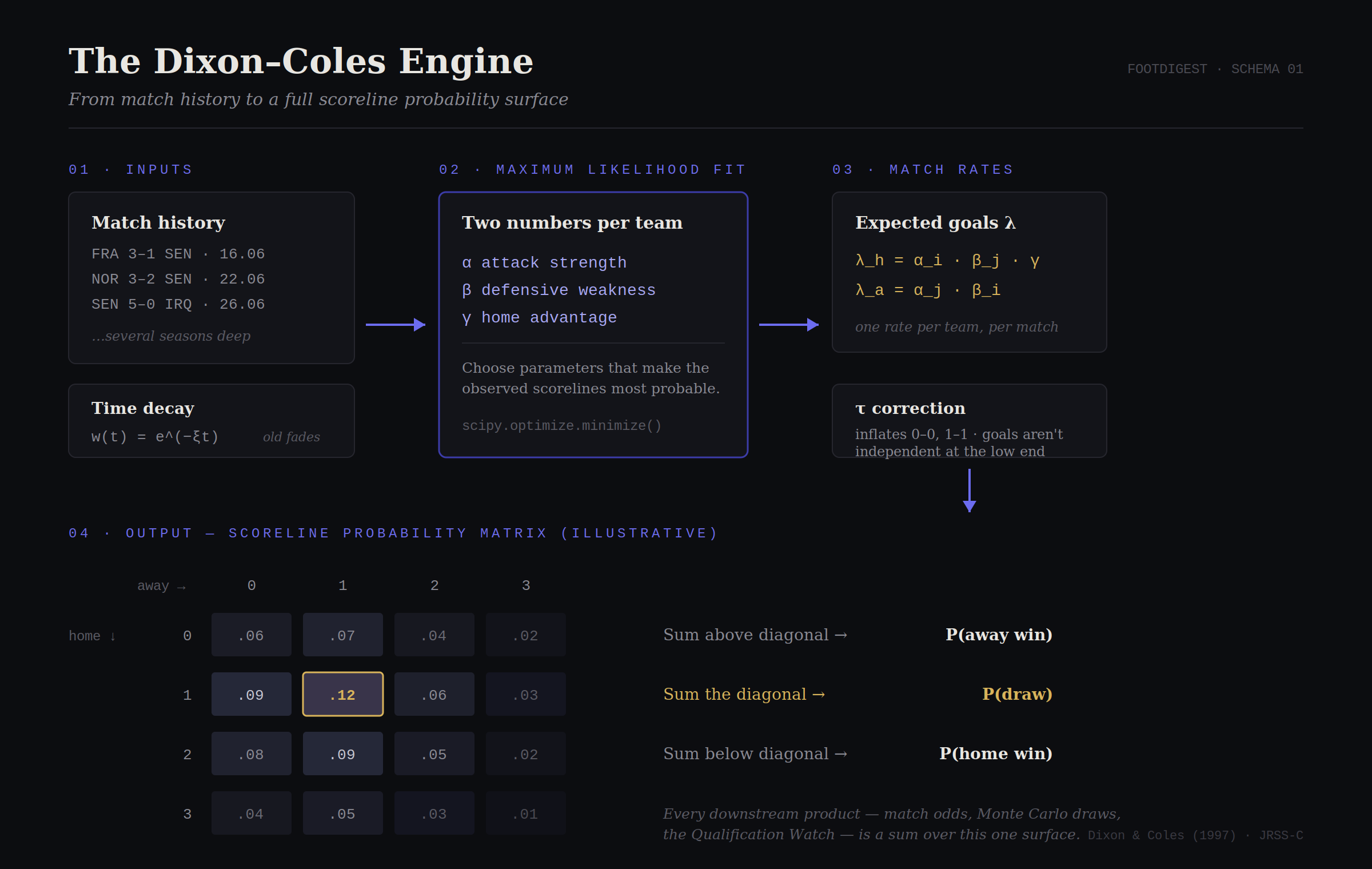
Figure 1: Move the ratings and watch the scoreline surface breathe. Every downstream probability in this paper is a sum over this one matrix.
II.2 · The rivals: bivariate Poisson and Elo
Rigour demands naming the alternatives and why FootDigest doesn’t use them.
Bivariate Poisson ( Karlis & Ntzoufras, 2003, JRSS-D [5] (2003). Analysis of Sports Data by Using Bivariate Poisson Models. JRSS-D 52. The principled alternative to τ. ) treats the two teams’ scores as sharing a common latent component, both counts get a joint “game tempo” shock, which models score correlation more elegantly than the τ patch. It fits better in-sample; out-of-sample forecasting gains over Dixon–Coles are consistently marginal, and the model is harder to fit and to explain. FootDigest’s design principle is that every modelling choice must be explainable in one paragraph on a team page. τ wins.
Elo (the chess rating adapted to football, and since 2018 the official basis of the FIFA World Ranking) is Dixon–Coles’s minimalist cousin: one number per team, updated after each match by K·(result − expected result). Its virtues are robustness and zero refitting. Its cost is silence: Elo predicts who wins but says nothing about scorelines, and scorelines are what you must sample to simulate group tables, tiebreakers, and goal difference. For tournament simulation, a goals model isn’t a preference. It’s a requirement.
II.3 · What the model actually said about Group I
Run through the fitted engine before the tournament, Senegal’s group read like a trap: France (elite α, elite β), Norway (a monstrous attack concentrated in one man, a walking violation of the constant-rate assumption named Haaland), Iraq (the group’s designated λ-donor). The model’s modal path for Senegal was precisely the one that occurred: competitive defeats to the two European sides, a heavy win over Iraq, third place, three points, and a prayer.
The 3–1 loss to France was almost a median simulation. Jackson struck the post; Ismaïla Sarr skied a six-yard chance just before half-time; Mbappé finished what he was given with the ruthlessness that makes him a one-man refutation of average rates. The scoreline said 3–1. The chance quality said something nearer a coin flip that France called correctly: a gap we will make precise in Part V, because that gap is the entire reason expected goals exists.
Pick any two teams and read the match. The ratings are illustrative, but the pipeline turning them into a scoreline (Elo supremacy into two goal rates, then the τ-corrected Dixon–Coles matrix) is the real model. It opens on Senegal vs Belgium: the 31% that started everything.
PART III: JUDGMENT
How to Score a Forecaster (Or: Why “You Predicted Wrong” Is Not an Argument)
Before simulating anything, an uncomfortable question: what does it even mean for a probabilistic forecast to be good? “The model said Senegal 62% and Senegal lost” is not a refutation, any more than surviving one round of Russian roulette refutes the danger. Single outcomes cannot falsify probabilities. Only populations of forecasts can. Three instruments make this precise, and they are FootDigest’s actual referee:
The Brier score: mean squared error between forecast probabilities and outcomes (1 if it happened, 0 if not). Lower is better. Punishes confidence in the wrong direction quadratically, which is exactly how it should feel.
The Ranked Probability Score (RPS): the football-specific standard, because home/draw/away outcomes are ordered: predicting a home win when the match is drawn is less wrong than predicting a home win when the away side wins. For cumulative forecast probabilities Fₖ and cumulative outcomes Oₖ over the ordered outcomes:
Set a forecast, pick the result, and watch the Brier and RPS penalties move. Being confident and wrong costs the most, which is exactly the point: one outcome cannot refute a probability, but a scoring rule can, in aggregate.
Calibration: the deepest of the three. Collect every match your model called ~70%, and check: did about 70% of them happen? Repeat across every probability band. A model is calibrated when its stated confidence matches its realized frequency everywhere. Calibration is the only sense in which a probabilistic model can be “right,” and it is checkable only in bulk: hundreds of matches, which is why FootDigest’s Dixon–Coles engine shipped only after backtesting across full seasons of historical fixtures, scored on RPS against a naïve baseline and against the one opponent that matters.
Illustrative. Drag the slider and watch a calibrated model bend into an overconfident one. A model is honest when its 70% predictions come true about 70% of the time: the closer the curve hugs the diagonal, the better.
That opponent is the betting market. Odds at kickoff, averaged across bookmakers and stripped of margin, are the strongest publicly available football forecast: a prediction market aggregating thousands of models and insiders. The professional standard for a model is brutal and simple: does it beat the closing line? Decades of the efficiency literature (Dixon and Coles’s own second act) say the answer is mostly no, occasionally, locally, yes, and any analytics product that won’t publish its scores against that benchmark is asking for faith, not offering evidence. FootDigest publishes its backtests. This paragraph is the reason.
PART IV: SIMULATION
Monte Carlo: Ten Thousand Senegals
IV.1 · The method born in a casino’s name
The Monte Carlo method was born at Los Alamos in the 1940s, when Stanisław Ulam (convalescing, playing solitaire) wondered about the probability of winning a given deal. The combinatorics were hopeless. His insight: just play a hundred hands and count. Nicholas Metropolis named the method after the casino where Ulam’s uncle gambled away the family money, which remains the most honest naming decision in the history of applied mathematics.
The principle: when a probability is too tangled to compute in closed form, simulate the world many times and count. The law of large numbers guarantees convergence, and the central limit theorem tells you how fast: the standard error of an estimated proportion p̂ over N simulations is
At N = 10,000, probabilities carry a standard error under half a percentage point. For a public-facing qualification tracker, that is precision to spare; the model’s systematic error dwarfs its sampling error, which brings us to the part most public simulators get silently wrong.
IV.2 · The two layers of uncertainty
A tournament simulation contains two distinct kinds of not-knowing, and conflating them is the cardinal sin of the genre:
Aleatoric uncertainty: the dice. Even with perfect ratings, match outcomes are random draws. This is the uncertainty the 10,000 simulations sample.
Epistemic uncertainty: the ratings themselves are estimates, fitted on finite, decaying data. Senegal’s “true” α is not a number my optimizer found; it is a number my optimizer approximated, with error bars. A rigorous pipeline propagates this by drawing the parameters, too, from their estimated distribution (or bootstrapped refits) before simulating each world. Otherwise your 4% is really “4%, conditional on my point estimates being exactly right,” which no one’s are. That is the ideal; FootDigest’s shipped engine samples only the first layer today (see Appendix A), and widening the headline to include the second is on the roadmap. The honest headline probability is wider than the naïve one, and honesty about width is a feature.
The pipeline, end to end:
- Fit Dixon–Coles on time-decayed international results.
- Draw a parameter vector from its uncertainty distribution.
- For every unplayed match, compute λ_home, λ_away, and draw a scoreline from the τ-corrected model. Not the most likely scoreline, a random one, in proportion to its probability. The distinction is everything: the modal scoreline in most matches is 1–1 at ~11%, and simulating only likely outcomes would erase precisely the chaos we are trying to measure.
- Apply the rules: group tables, head-to-head tiebreakers, goal difference, the eight-best-thirds ranking, the bracket. This step is the unglamorous mass of the codebase, hundreds of lines transcribing FIFA’s regulations, and it is where most public models silently fail. A simulator that draws beautiful Poisson scorelines and then botches the third-place tiebreaker is a beautiful lie.
- Repeat 10,000 times. Count.

Figure 2: Press the button. Ten thousand worlds, counted. The seed is yours to change; the convergence is not. (Illustrative group, not the live engine.)
Now the whole tournament. An illustrative 16-team knockout, seeded by illustrative Elo and run thousands of times, so both raw strength and bracket luck shape each team’s title odds. Senegal is highlighted. Watch the bars reorder as the count climbs. Not the live engine.
IV.3 · June 26th, as a probability current
Now watch the machinery meet reality. After the group stage Senegal held three points, +2 goal difference, and a fate entirely in other groups’ hands, dependent on final results in Groups G, H, J, K and L. This is not a scenario human intuition can price. It is a conditional probability tree collapsing branch by branch, live:
The Qualification Watch was recomputing scenarios faster than I could write commentary about them.
Each result was a measurement collapsing the wave function of Senegal’s tournament. By Friday night, ten thousand simulated Senegals had become one real one: through to the Round of 32 as the only third-place side on three points, an outcome my pre-tournament runs had placed in roughly one world in twenty-five. Rare, but represented. The entire point of Monte Carlo is that a few hundred of your simulated futures were already living there, waiting for reality to pick.
And this is the deeper lesson simulation teaches, the one I return to every time I write about Senegal for a Senegalese audience: a team’s tournament is not a fact; it is a distribution. The Senegal eliminated by Belgium in extra time and the Senegal that reached the quarter-finals coexisted, at meaningful probability, until roughly 11pm Seattle time on July 1st. Supporters live inside one sampled path. Models live in all of them at once. Grief is what it feels like to be forced from the second view back into the first.
PART V: THE GEOMETRY OF A MOMENT
Expected Goals as Trigonometry With a Win Rate
V.1 · The visible angle
Descend from tournaments to a single instant. First half, June 16th, New York. Nicolas Jackson, low shot from the left, off the post, off Mike Maignan’s leg, out for a corner. The scoreboard registers nothing. What should it have registered?
Expected goals (xG) answers a precisely posed question: of all historical shots taken from this situation, what fraction became goals? A shot’s xG is that learned probability. And before any machine learning arrives, xG is geometry: specifically, the geometry a striker’s nervous system evaluates in two hundred milliseconds and a model computes explicitly.
Two variables dominate everything. Distance: scoring probability decays steeply, roughly exponentially, as you retreat from goal. The visible angle: the goal mouth is 7.32 metres wide, and the angle it subtends from your position is, functionally, how open the door is. From a point x metres out from the goal line and y metres lateral of centre, the subtended angle has a closed form (a direct application of the tangent difference identity):
From the penalty spot, θ ≈ 36°. Drift toward the byline and θ collapses toward zero, the goal geometrically closes. Plot the level curves of θ on a pitch and you get nested arcs radiating from the goal mouth: a probability field, invisible but as real as the grass. Elite strikers are, functionally, gradient-ascent algorithms on this field. Watch Mbappé’s movement in the Norway–France group decider and you are watching someone surf the contours toward the region where θ is fat and defenders are absent.
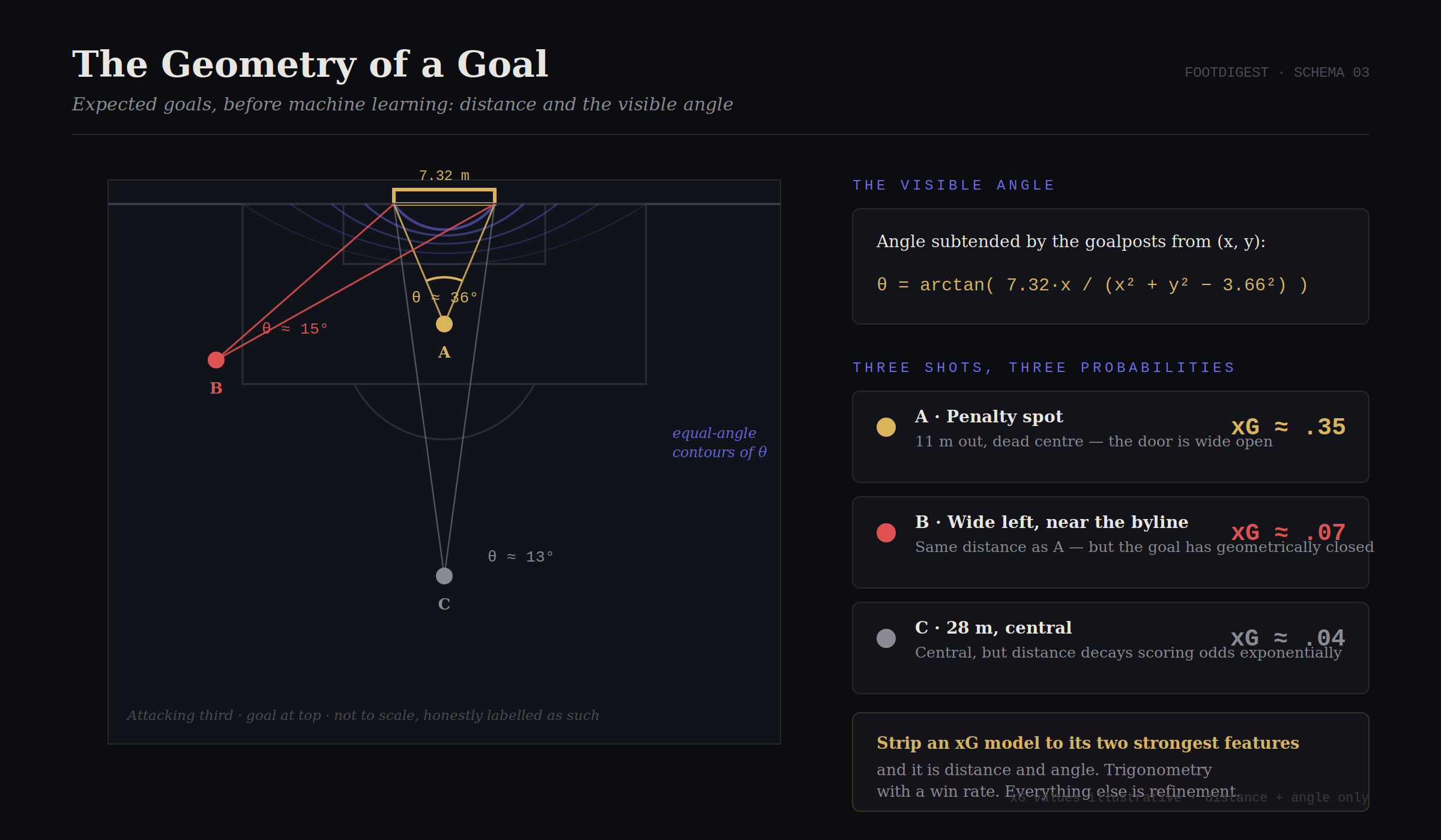
Figure 3: Drag the shot. Distance decays your chances; the visible angle closes the door. Trigonometry with a win rate.
V.2 · From geometry to learning
The first xG models were logistic regressions: probability of a goal = σ(w₀ + w₁·distance + w₂·angle + …), where σ is the sigmoid squashing any real number into (0,1). Modern versions are gradient-boosted tree ensembles adding body part, assist type, defensive pressure, counter-attack state, goalkeeper position, and, where tracking data exists, the full defensive geometry at the moment of the shot. But strip any provider’s model to its two strongest features and you recover distance and angle. Everything since 2012 is refinement of a trigonometric core.
Three rigour notes the highlight-reel discourse always omits:
xG models disagree with each other. Different providers, different training data, different feature sets: the same shot can be 0.31 to one model and 0.42 to another. An xG value without its provider is a number without units. FootDigest displays sources on every figure for exactly this reason.
Shot selection bias. The model learns from shots taken. But who shoots from bad positions? Disproportionately, players with no better option, or unusual confidence in that skill. The training data is not a random sample of situations; it is a sample filtered through professional judgment, and the model quietly inherits that filter.
A single match’s xG is noisy. Summing a handful of Bernoulli probabilities inherits all the variance of Part I. The value of xG is longitudinal: across many matches, chance creation persists while finishing luck mean-reverts, which is why a team’s xG history predicts its future results better than its actual results do. This is the statistical argument for judging performances rather than scorelines, and it is the hill FootDigest’s editorial line dies on. Senegal’s group stage produced three points; its chance-quality profile was worth more. Belgium discovered as much for ninety-three minutes. Mathematics offers no consolation prizes, but it does write accurate epitaphs.
PART VI: THE VALUE OF EVERYTHING ELSE
Markov Chains and the Price of a Pass
xG has one enormous blind spot: it prices only shots. But most of football is not shooting: it is the patient manufacture of shooting positions. What is a line-breaking pass from midfield worth? What did Habib Diarra’s carry through Iraq’s midfield contribute, three actions before anyone shot? The modern answer borrows the central object of stochastic process theory: the Markov chain.
Model a possession as a walk between states: zones of the pitch, plus two absorbing states, goal and possession lost. The Markov property assumes the future depends only on the present state, not the path that led there (false in detail, useful in bulk, like every good assumption in this paper). Then define the value of every zone z as the probability that a possession currently in z eventually produces a goal. This satisfies a self-consistency equation. Readers from reinforcement learning will recognize the Bellman equation immediately:
The value of where you stand = the chance you score from here, plus the expected value of everywhere you might move the ball next. Estimate the transition probabilities by counting millions of historical actions, solve the fixed point, and the pitch acquires a value surface: near zero in your own corner, swelling through midfield, steepening sharply inside the box.
Now the beautiful move. The value of a pass, of any action, is the difference it makes:
This is Expected Threat (xT), popularized in Karun Singh’s 2019 formulation [11] (2019). Introducing Expected Threat (xT). The value-surface formulation that made Markov possession value a public language. , with intellectual roots in Sarah Rudd’s 2011 Markov framework [10] (2011). A Framework for Tactical Analysis and Individual Offensive Production Assessment in Soccer Using Markov Chains. NESSIS. Possession as a Markov process, years ahead of its industry. , work she presented years before joining a Premier League club’s front office. Its academic sibling, VAEP ( Decroos et al., KDD 2019 [12] (2019). Actions Speak Louder than Goals: Valuing Player Actions in Soccer. KDD 2019. VAEP; every action priced in both directions. ), extends the idea to all on-ball actions and both directions of play: every touch is scored by how much it raises your probability of scoring and lowers your probability of conceding, within the next few actions.
The consequence is a quiet revolution in who gets credit. Goals and assists reward the last two touches of a move; xT and VAEP pay the invisible labour: the fullback’s switch that flipped the value surface, the midfielder’s half-turn between the lines. When FootDigest’s match reports insist a deep-lying midfielder was the match’s decisive player despite a blank scoresheet, this fixed-point equation is what’s doing the insisting.
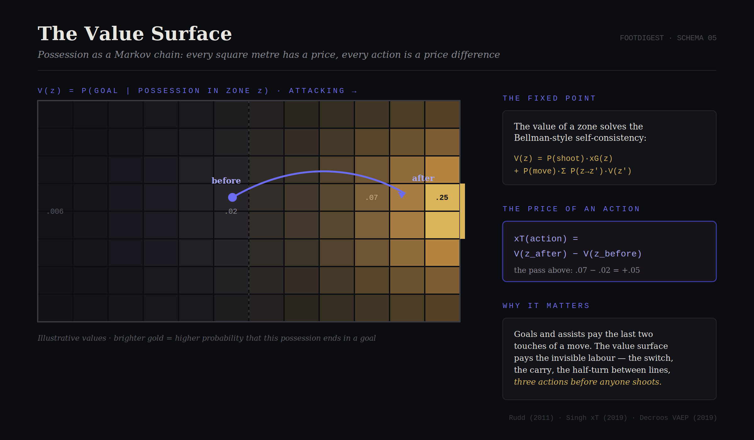
Figure 4: Tap two zones to price a pass: the difference between where the ball was and where it is now. (Illustrative surface.)
PART VII: THE GEOMETRY OF SPACE
Voronoi, Pitch Control, and Football as a Graph
Everything so far prices events: goals, shots, passes. But coaches do not think in events; they think in space. And space has been rigorously mathematized.
VII.1 · Who owns the pitch
At any frozen instant, which player controls which region? The first-order answer is a Voronoi tessellation: assign every point of the pitch to its nearest player. Formally, player p’s cell is
The pitch shatters into 22 convex polygons, and tactics becomes visible geometry. A compact low block: tiny defensive cells, starving the opponent of central polygons. A stretched transition: vast unguarded cells behind the fullbacks, precisely the acreage Belgium’s substitutes flooded during those three minutes in Seattle, when Senegal’s block, protecting its lead, dropped ten metres and ceded the midfield polygons entirely. (Part X returns to why protecting a lead invites this; the geometry and the probability theory of it are the same fact viewed from two sides.)
Raw Voronoi assumes all players are equally fast, currently stationary, and infinitely attentive. William Spearman’s [13] (2018). Beyond Expected Goals. MIT Sloan Sports Analytics Conference. Pitch control: physics-aware ownership of space. pitch control model (developed at Liverpool FC; Beyond Expected Goals, Sloan 2018) repairs this physically: for every point, compute the probability that each team would arrive first if the ball were played there, folding in current velocities, acceleration limits, and the ball’s own travel time. The output is a continuous ownership probability surface over the pitch, refreshed at tracking-data frequency (25 Hz). Fernández and Bornn’s Wide Open Spaces (Sloan 2018) [14] (2018). Wide Open Spaces. MIT Sloan Sports Analytics Conference. Space valued by threat, closing the loop between Parts VI and VII. closes the loop by weighting controlled space by its value: space is only worth what the value surface of Part VI says it threatens.
VII.2 · The team as a graph
From the same tracking and event data, further geometric objects fall out:
- Convex hulls, the smallest polygon containing a team’s outfield players: hull area measures compactness (pressing teams shrink it; possession teams inflate it), and the hull centroid’s height measures collective courage.
- Passing networks: players as nodes, pass frequencies as weighted edges, and suddenly sixty years of graph theory applies for free. Betweenness centrality identifies the metronome: remove De Bruyne’s node and Belgium’s network loses most of its throughput. Clustering coefficients expose triangle play. And the entropy of the pass distribution measures unpredictability: great attacking teams are high-entropy objects, expensive to compress and therefore expensive to defend.
Here is what I find quietly profound: formations were always graphs, and tactics were always geometry: we merely lacked the sensors. “4-4-2” is a lossy, human-readable compression of a 22-node dynamic graph sampled 25 times per second. When a commentator says a side is “compact between the lines,” there is now a polygon area and a cell-size distribution for that. Cruyff’s vocabulary and computational geometry’s vocabulary turn out to be the same language in two notations, separated by fifty years of missing instrumentation.
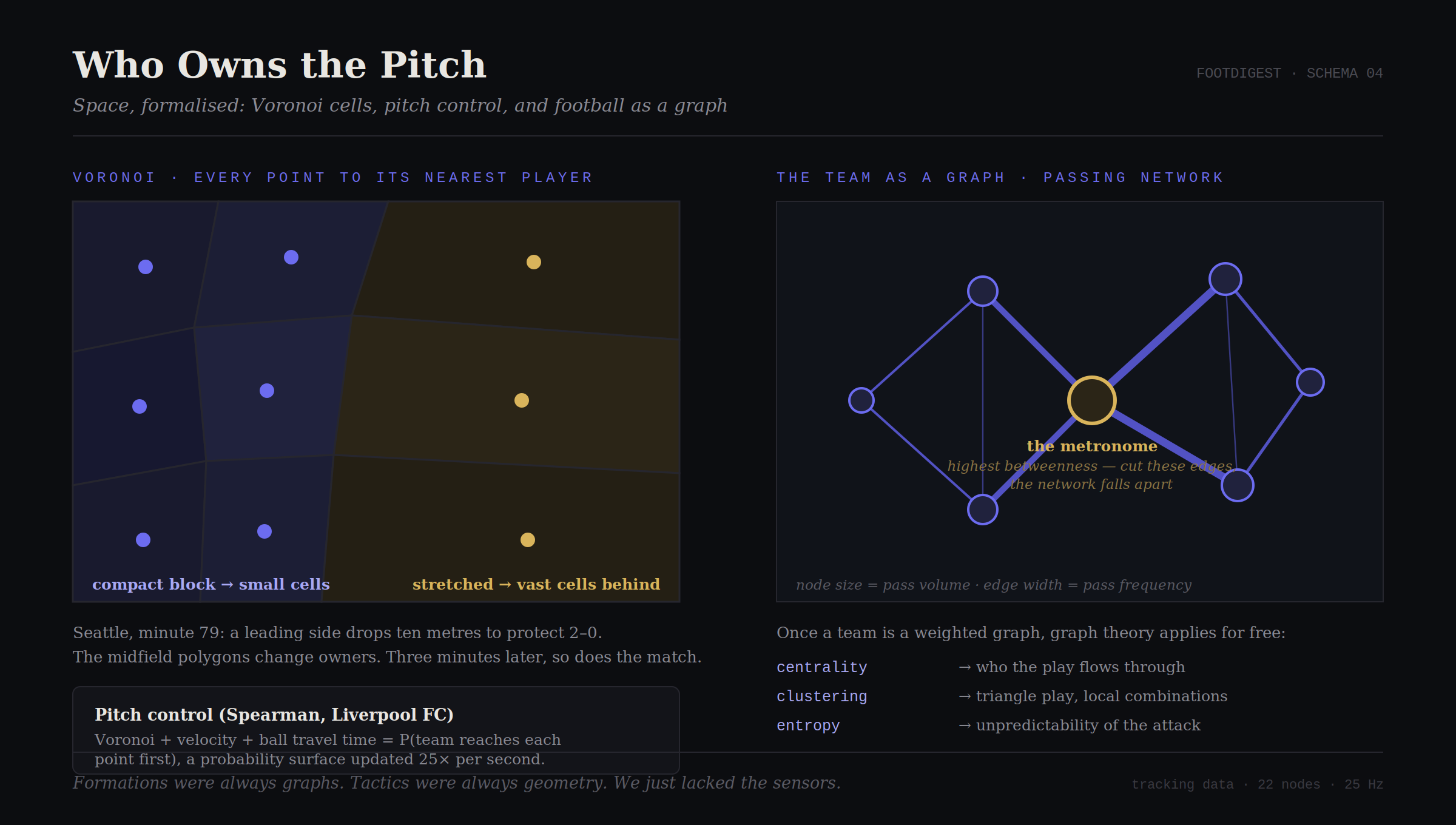
Figure 5: Drag any player and the ownership map reflows. Load the “Seattle, minute 79” preset to watch a protected lead cede the midfield polygons.
PART VIII: GAME THEORY AT ELEVEN METERS
The Only Place in Sport Where a 1928 Theorem Is Tested Weekly
On the night of June 29th, this World Cup staged a controlled experiment. Morocco 1–1 Netherlands, penalties: Morocco through, 3–2. Germany 1–1 Paraguay, penalties: Paraguay through, 4–3. Two shootouts, two eliminated giants, one night, and underneath both, the cleanest real-world laboratory that exists for John von Neumann’s minimax theorem.
A penalty kick is a nearly ideal two-player zero-sum game. The kicker chooses a side; the keeper, forced by ball flight times of ~0.3 seconds against human reaction times, must commit essentially simultaneously. Simplify both players’ choices to and the logic of the mixed-strategy equilibrium bites immediately: if you kick to your natural side too often, keepers exploit it; any pattern is a leak. Von Neumann’s 1928 theorem says the optimal play is a precisely calibrated randomization: mix your choices so that your opponent’s expected payoff is identical whichever way they dive, leaving them nothing to exploit. The equilibrium mix is not 50/50; it depends on your scoring probabilities in each cell of the payoff matrix (kickers are stronger to their natural side, so the equilibrium leans natural, but only leans).
What elevates this from textbook example to empirical science is that professional footballers were tested against the theorem, and passed. Ignacio Palacios-Huerta (Review of Economic Studies, 2003) [7] (2003). Professionals Play Minimax. Review of Economic Studies 70. Penalty kicks as an empirical test of von Neumann; professionals pass. assembled over a thousand professional penalties and checked minimax’s two sharp predictions: (1) a kicker’s scoring probability should be statistically identical across his strategies (if kicking left scored more than kicking right, he should kick left more until the margin closes) and (2) choice sequences should be serially independent, patternless, unexploitable. Both held. A parallel study by Chiappori, Levitt and Groseclose (American Economic Review, 2002) [8] (2002). Testing Mixed-Strategy Equilibria When Players Are Heterogeneous. AER 92. Independent confirmation on French and Italian penalties. reached the same conclusion on French and Italian data. Professional footballers, most of whom have never heard the word “minimax,” play one of the few known human approximations of exact game-theoretic equilibrium, because for a century, deviation has been ruthlessly selected against. The theory works here precisely because the money and the Darwinism are real.
And then, a cautionary coda in the same literature, a replication story every data person should tattoo somewhere. Apesteguia and Palacios-Huerta (AER, 2010) [9] (2010 / 2012). Psychological Pressure in Competitive Environments. AER 100; Management Science 58. The first-kicker advantage and its contested replication; read as a pair. reported that the team kicking first in a shootout wins about 60% of the time: a psychological-pressure effect, widely publicized, which prompted FIFA to trial the “ABBA” kicking order. Subsequent studies on larger samples (notably Kocher, Lenz and Sutter in Management Science, 2012 [9] (2010 / 2012). Psychological Pressure in Competitive Environments. AER 100; Management Science 58. The first-kicker advantage and its contested replication; read as a pair. ) found the advantage shrank toward statistical insignificance. The current honest summary: the first-kicker edge is plausible, small, and contested, and the episode is football analytics’ own replication crisis in miniature. One dataset’s 60% is another dataset’s coin flip. FootDigest’s sourcing rule exists because of stories exactly like this one.

Figure 6: Take ten penalties against a keeper that learns your patterns. Then read why your only defence was a coin you weren’t flipping. (Payoffs illustrative.)
PART IX: LEARNING MACHINES
From Counting to Watching
Everything so far is statistics on events. The frontier is learning on trajectories: models that ingest raw positional data and understand the game the way a coach’s eye does. A taxonomy of where the field genuinely stands, ranked by maturity:
Gradient-boosted trees (XGBoost, LightGBM) remain the workhorses of every tabular problem: xG, outcome classification, action valuation. Unreasonably effective, cheap, and interpretable enough to argue with, which in a coaching environment is not a nicety but a deployment requirement.
Graph neural networks treat the 22 players as nodes carrying positions and velocities, and learn functions respecting the game’s symmetries. The landmark is DeepMind’s TacticAI ( Wang et al., Nature Communications, 2024 [15] (2024). TacticAI: an AI assistant for football tactics. Nature Communications 15, 1906. Geometric deep learning on 7,176 corners; the 90% preference result and its five-rater caveat. ), built with Liverpool FC on 7,176 Premier League corner kicks: it predicts the corner’s receiver, predicts whether a shot follows (F1 ≈ 0.71), and, the generative leap, proposes adjusted defensive setups that reduce the shot probability. In blind evaluation, Liverpool’s staff preferred TacticAI’s suggested arrangements over the setups actually used 90% of the time. Rigour footnote, because this paper promised rigour: that signature 90% comes from five expert raters at a single club: genuinely impressive, and genuinely narrow, and both of those facts belong in the same sentence. Set pieces, being semi-static, were the natural first conquest. Open play is the war.
Sequence models, the transformer architecture behind the current AI wave, are being pointed at possession sequences, learning the grammar of attacks the way language models learn sentences. The tantalizing application is counterfactual: given this build-up, what would a typical elite side have played next? The divergence between the actual pass and the model’s predicted distribution becomes a measurable definition of creativity: Iliman Ndiaye’s decision-making, expressed as distance from the expected.
And a confession of craft, because I build production systems for a living in my other life: the model is never the hard part. The hard part is the pipeline: ingesting feeds, reconciling provider IDs, surviving the abandoned match and the postponed kickoff, versioning ratings so that Tuesday’s article and Thursday’s article cannot silently disagree. FootDigest runs on the same engineering discipline as the health-data infrastructure I’ve built for governments: idempotent jobs, immutable audit trails, and the product rule already stated twice because it is the whole constitution: real sourced numbers or honest absence. In football analytics, as in public infrastructure, you lose the room with the first number you cannot defend.
PART X: WHERE THE MATHEMATICS ENDS
Return, finally, to Seattle, because I owe you the end of that story, and because the ending is the most mathematically interesting part of this entire tournament.
Senegal 2, Belgium 0, minute 79, the kind of lead that, historically, survives better than nine times in ten. Then two goals in three minutes. Anyone who has fit in-play models knows the constant-rate Poisson assumption dies precisely here, and dies in a measured way: scoring intensity is state-dependent. A team trailing late in a knockout match attacks with reallocated risk; the leading team’s block drops; λ becomes λ(state, time), rising for the desperate side exactly when the game matters most, the well-documented score effects of the in-play literature. Simultaneously, Part VII’s geometry tells the same story from the other side: the deeper block cedes the midfield Voronoi cells, pitch control migrates toward the trailing team, and the value surface under their possessions swells. The probability theory and the geometry are one phenomenon wearing two notations. A properly state-dependent model gave Belgium more than the naïve model did, and still only a slim path. Belgium took it.
Then extra time, and a penalty of the kind no feature vector on Earth encodes: a referee’s judgment at the boundary of interpretability, reviewed, upheld, decisive. The temptation is to say the mathematics failed. It did not. The mathematics said rare, and rare is not impossible, and the distance between those two words is where football lives.
So let me close the technical part of this paper with its three most important sentences, each earned the hard way:
1. Calibration is the only virtue, and it is cold comfort. A good model is not one that “picked the winner”; it is one whose 70% predictions come true 70% of the time, verifiable only across hundreds of matches via the scoring rules of Part III. On any single night, in any single stadium, a perfectly calibrated model can and will watch its favourite die. It is designed to.
2. The tails belong to humans. Penalties awarded and penalties missed, red cards, VAR interventions, a goalkeeper’s leg redirecting Jackson’s shot onto the post rather than inside it: these live in the residual, the variance no feature explains. The best match-outcome models today, mine included, leave the majority of result variance unexplained. That residual is not a failure of method. That residual is the game.
3. A distribution is not a destiny. Fatalism cuts both ways, and both are misuses of the maths. After Senegal lost their opening two games (to France, then Norway) the living rooms in Dakar had already buried them; the model, unsentimental about the eight-best-thirds arithmetic, still made them better than a two-in-three bet to go through, and they did, five-nil over Iraq with survival on the line. The opposite error is worse: reading a single-digit probability as a zero. South Africa reached the knockouts for the first time in their history. Group G reordered itself seven times in an evening, the last time by a VAR line’s width. Every one of those was a tail event. Tails are not the failure mode of football. Tails are the product.
Coda: 2002, and Why I Build
There is a match my model never saw, because it predates my data’s decay horizon by two decades: May 31st, 2002. Senegal 1, France 0. The reigning world champions, beaten in the opening match of the World Cup by a debutant nation. Every Senegalese of my generation carries that scoreline like a birthmark. When this June’s draw produced France–Senegal, the first competitive meeting since, no parameter in any model on Earth encoded what the fixture meant.
That is the point, in the end. The mathematics does not replace the meaning; it gives the meaning a spine. When the Qualification Watch keeps faith in your team at zero points, trusting the eight-best-thirds arithmetic the whole neighbourhood had given up on, and the maths is vindicated, the joy is not smaller for having been quantified; it is sharper, because you knew the door was wider than the grief in the room believed. And when the tail arrives wearing red, in extra time, in Seattle, the grief is real and the model is intact, and a grown person is allowed to hold both.
Poisson gives us the randomness, and Ben-Naim gives us its measure. Dixon–Coles gives us the ratings; Brier and RPS keep them honest. Monte Carlo gives us the futures, both layers of them. Trigonometry prices the shot; Markov prices everything before it; Voronoi maps the ground it happens on; von Neumann governs its final, loneliest form. Machine learning gives us eyes we did not have. And football (stubborn, low-scoring, measurably the least predictable great game humans have invented) gives us the reason to keep computing.
Beyond scores. Football, distilled.
Appendix A: The FootDigest Model Card
A prediction you cannot audit is an opinion with extra steps. Specification of the engine behind every probability in this paper:
Model class. An Elo-driven Dixon–Coles scoreline model: team strength is a single World-Football-Elo rating; the rating gap becomes a goal supremacy that splits into two Poisson goal rates, corrected on the low-score cells by the Dixon–Coles factor τ. Tournament outcomes come from Monte Carlo group simulation over that scoreline model.
Parameters. One Elo rating per team (start 1500, K-factor 40, +100 on non-neutral home ground, goal-difference multiplier). Scoreline mapping: baseline 2.6 goals, 170 Elo points per goal of supremacy, low-score dependence ρ = −0.1. Host advantage applied only at non-neutral venues.
Training data. The martj42/international_results open dataset (CC0): every scored senior men’s international, 1872–present (≈49,400 matches at time of writing), all competitions, mirrored and re-synced daily.
Estimation. Elo ratings are updated online after every match (a point estimate, recomputed from full history on each dataset sync); the Dixon–Coles constants are fixed, not fitted. A time-weighted, maximum-likelihood-fitted attack/defence Dixon–Coles was evaluated as an alternative and did not out-perform the Elo strength model out-of-sample, so the simpler model ships.
Simulation. 1,000 seeded Monte Carlo group completions per update; full FIFA 2026 regulations, including the eight-best-thirds ranking and all tiebreakers. Reported probabilities carry Monte Carlo sampling noise only: parameter uncertainty is not propagated.
Validation. Backtested out-of-sample on the 2,607 internationals played since 1 January 2024 (trained only on prior matches): RPS 0.173 vs. a naïve base-rate baseline of 0.227, a 24% reduction; calibration is monotonic with mild over-confidence on strong home favourites. A market (betting-odds) benchmark and a neural-net comparison are not reported: that data is not in the system, and I won’t quote a number I can’t compute.
Known failure modes. Team strength is a single scalar (no fitted per-team attack/defence split) with no recency time-decay; state-dependent late-game intensity is unmodelled (it systematically underweights trailing-team surges, see Seattle); squad shocks (injuries, suspensions) enter only through Elo drift; there is no within-match, player-level information.
In-play win probability (research prototype). The minute-by-minute path in the opening figure is not produced by the shipped engine, which carries no within-match information (above). It was computed offline from live match-insight data, conditioning the pre-match scoreline model on the running score and the minutes remaining — a prototype of an in-play feature I intend to build into FootDigest, shown here for illustration, not as a live capability.
(Every number in this card is measured from the live engine or its backtest; the one quantity computed offline, the opening in-play path, is flagged as a prototype directly above. Real sourced numbers, honest absence for what the data can’t yet support.)
Appendix B: Annotated Bibliography
- Moroney, M.J. (1956). Facts from Figures. Penguin. The first serious statistical treatment of football scores; Poisson and negative binomial fits.
- Reep, C. & Benjamin, B. (1968). “Skill and Chance in Association Football.” JRSS-A 131. The founding paper and the founding fallacy; read it alongside its critics as a permanent vaccine against denominator neglect.
- Maher, M.J. (1982). “Modelling Association Football Scores.” Statistica Neerlandica 36. Attack/defence Poisson structure; the skeleton of everything since.
- Dixon, M.J. & Coles, S.G. (1997). “Modelling Association Football Scores and Inefficiencies in the Football Betting Market.” JRSS-C 46. The workhorse: τ correction, time decay, and a demonstration of market inefficiency in one paper.
- Karlis, D. & Ntzoufras, I. (2003). “Analysis of Sports Data by Using Bivariate Poisson Models.” JRSS-D 52. The principled alternative to τ.
- Ben-Naim, E., Vazquez, F. & Redner, S. (2006). “Parity and Predictability of Competitions.” J. Quantitative Analysis in Sports 2(4). 300,000+ matches; football measured as the major sport with the highest upset frequency.
- Palacios-Huerta, I. (2003). “Professionals Play Minimax.” Review of Economic Studies 70. Penalty kicks as an empirical test of von Neumann; professionals pass.
- Chiappori, P-A., Levitt, S. & Groseclose, T. (2002). “Testing Mixed-Strategy Equilibria When Players Are Heterogeneous.” AER 92. Independent confirmation on French and Italian penalties.
- Apesteguia, J. & Palacios-Huerta, I. (2010). “Psychological Pressure in Competitive Environments.” AER 100; and Kocher, M., Lenz, M. & Sutter, M. (2012), Management Science 58. The first-kicker advantage and its contested replication; read as a pair.
- Rudd, S. (2011). “A Framework for Tactical Analysis and Individual Offensive Production Assessment in Soccer Using Markov Chains.” NESSIS. Possession as a Markov process, years ahead of its industry.
- Singh, K. (2019). “Introducing Expected Threat (xT).” The value-surface formulation that made Markov possession value a public language.
- Decroos, T. et al. (2019). “Actions Speak Louder than Goals: Valuing Player Actions in Soccer.” KDD 2019. VAEP; every action priced in both directions.
- Spearman, W. (2018). “Beyond Expected Goals.” MIT Sloan Sports Analytics Conference. Pitch control: physics-aware ownership of space.
- Fernández, J. & Bornn, L. (2018). “Wide Open Spaces.” MIT Sloan Sports Analytics Conference. Space valued by threat, closing the loop between Parts VI and VII.
- Wang, Z. et al. (2024). “TacticAI: an AI assistant for football tactics.” Nature Communications 15, 1906. Geometric deep learning on 7,176 corners; the 90% preference result and its five-rater caveat.
The FootDigest Dixon–Coles engine, its full backtests, and the Qualification Watch methodology get their own technical companion post, with code, if enough of you ask. You know where the button is.
Errata & updates
No corrections yet.